Sample Reordering

This tutorial uses the Human Microbiome Project 2 data available from the HMP2Data library to demonstrate the functionality of the reorder_samples_by function in microshades.

Load packages

Load the necessary packages for this tutorial.

HMP2 data is provided as phyloseq, SummarizedExperiment, and MultiAssayExperiment class objects, so the corresponding packages need to be installed and/or loaded.

library(microshades)
library(phyloseq)
library(ggplot2)
library(dplyr)
library(cowplot)
library(forcats)
library(tidyverse)

library(HMP2Data)             # BiocManager::install("HMP2Data")
library(SummarizedExperiment) # BiocManager::install("SummarizedExperiment")
library(MultiAssayExperiment) # BiocManager::install("MultiAssayExperiment")

Load and prepare data

ps_momspi16S <- momspi16S()

ps_momspi16S

## phyloseq-class experiment-level object
## otu_table()   OTU Table:         [ 7665 taxa and 9107 samples ]
## sample_data() Sample Data:       [ 9107 samples by 13 sample variables ]
## tax_table()   Taxonomy Table:    [ 7665 taxa by 7 taxonomic ranks ]

The ps_momspi16S object contains 9,107 samples. Subset this data to focus on a smaller sample size:

ps_momspi16S_sub <- subset_samples(ps_momspi16S, 
                                   sample_body_site == "vagina")

ps_momspi16S_sub <- subset_samples(ps_momspi16S_sub, 
                                   visit_number %in%c(3,9))

Here we create a new column with shortened subject IDs, by taking the last three characters of each.

We will keep samples corresponding to a select list of shortened subject IDs.

These steps are for ease of use in later sections of this tutorial.

subj_ids <- sample_data(ps_momspi16S_sub)$subject_id

sample_data(ps_momspi16S_sub)$short_subject_id <- substr(subj_ids, 
                                                         nchar(subj_ids) - 2, 
                                                         nchar(subj_ids))

select_ids <- c("21e", "698", "124", "7f1", 
                "571", "004", "f61", "d96",
                "803", "44e", "a53", "760", 
                "7e1", "e7f", "fc8", "a7d", 
                "dc4", "10e", "fce", "54e", 
                "112")

ps_momspi16S_sub <- subset_samples(ps_momspi16S_sub, short_subject_id %in% select_ids)

Apply microshades functions

Use the prep_mdf and create_color_dfs microshades functions to evaluate abundance and apply advanced color organization.

# Use microshades function prep_mdf to agglomerate, normalize, and melt the phyloseq object
mdf_momspi16S <- prep_mdf(ps_momspi16S_sub,
                          subgroup_level = "Genus")

# Create a color object for the specified data
color_objs_momspi16S <- create_color_dfs(mdf_momspi16S, 
                                         selected_groups = c('Proteobacteria', 'Actinobacteria', 
                                                              'Bacteroidetes', 'Firmicutes'),
                                         group_level = "Phylum",
                                         subgroup_level = "Genus",
                                         cvd = TRUE)

# Extract plotting objects
mdf_momspi16S <- color_objs_momspi16S$mdf
cdf_momspi16S <- color_objs_momspi16S$cdf

Order based on taxon at group level

Note: in the following examples, subgroup_level is Genus and group_level is Phylum.

First, subset to a single visit to focus the view further.

ps_momspi16S_v3 <- subset_samples(ps_momspi16S_sub, visit_number == 3)

# Use microshades function prep_mdf to agglomerate, normalize, and melt the phyloseq object
mdf_momspi16S_v3 <- prep_mdf(ps_momspi16S_v3,
                             subgroup_level = "Genus")

# Create a color object for the specified data
color_objs_momspi16S_v3 <- create_color_dfs(mdf_momspi16S_v3,
                                            selected_groups = c('Proteobacteria', 'Actinobacteria', 
                                                                'Bacteroidetes', 'Firmicutes'),
                                            group_level = "Phylum",
                                            subgroup_level = "Genus",
                                            cvd = TRUE)

# Extract plotting objects
mdf_momspi16S_v3 <- color_objs_momspi16S_v3$mdf
cdf_momspi16S_v3 <- color_objs_momspi16S_v3$cdf

It is important to note that any specification of the order_tax parameter must match either group_level or subgroup_level, set during creation of the mdf and cdf objects (see above).

Here, we order based on a specific phylum (group level). The following plot is ordered by abundance of the phylum Actinobacteria.

color_objs_reorder_ab <- reorder_samples_by(mdf_momspi16S_v3,
                                            cdf_momspi16S_v3,
                                            order_tax = "Actinobacteria")

mdf_reorder_ab <- color_objs_reorder_ab$mdf
cdf_reorder_ab <- color_objs_reorder_ab$cdf

The reorder_samples_by function returns color objects, which must be extracted to then use with the plot_microshades function.

hmp_legend_1 <- custom_legend(mdf_reorder_ab, cdf_reorder_ab)

hmp_plot_1 <- plot_microshades(mdf_reorder_ab, cdf_reorder_ab) +
  scale_y_continuous(labels = scales::percent, expand = expansion(0)) +
  theme(legend.position = "none") +
  theme(axis.text.x = element_text(size= 8)) +
  theme (strip.text.x = element_text(size = 8))


plot_grid(hmp_plot_1, hmp_legend_1, rel_widths = c(1, .25))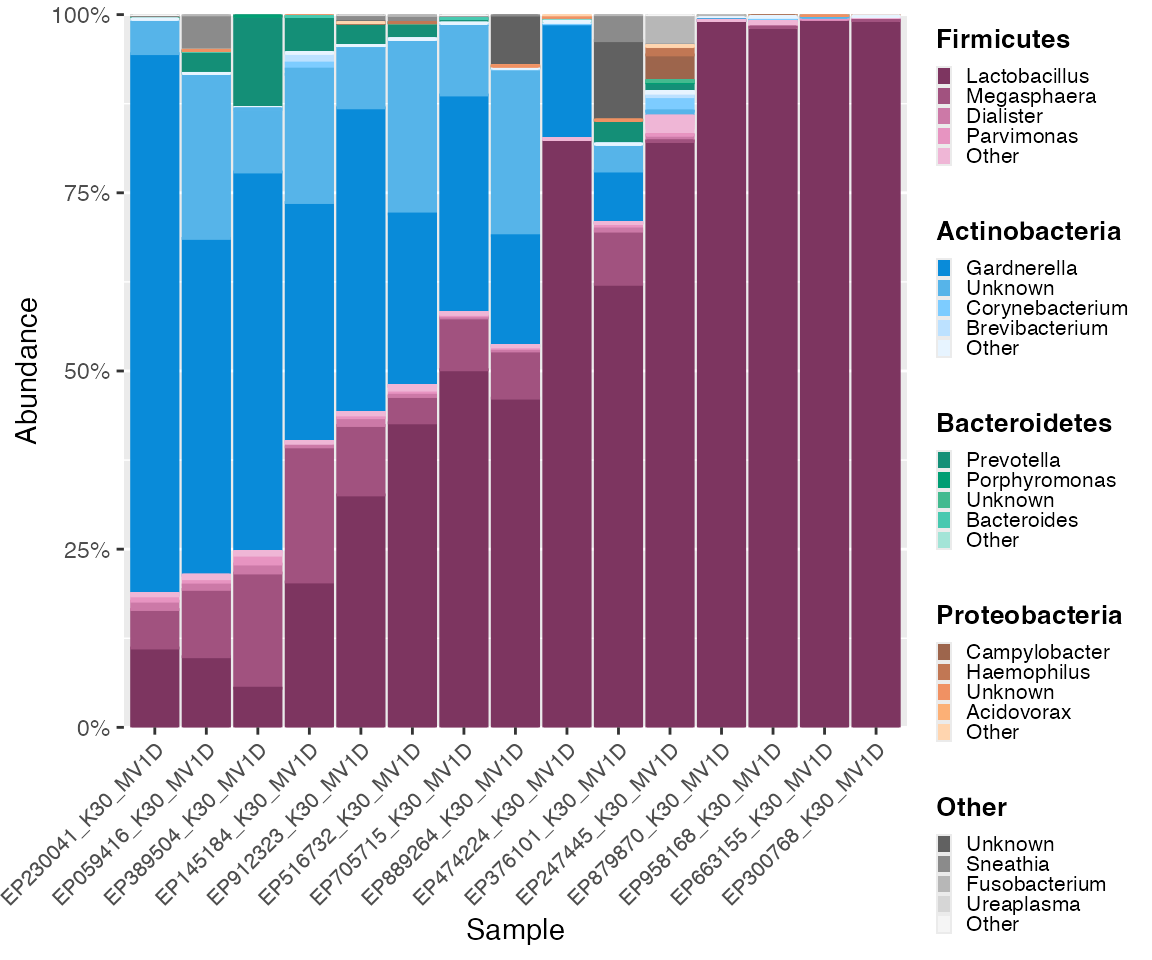

Order based on taxon at subgroup level

Here, we order based on a specific genus (subgroup level). The following plot is ordered by abundance of the specified genus Lactobacillus.

color_objs_reorder_lb <- reorder_samples_by(mdf_momspi16S_v3,
                                            cdf_momspi16S_v3,
                                            order_tax = "Lactobacillus")

mdf_reorder_lb <- color_objs_reorder_lb$mdf
cdf_reorder_lb <- color_objs_reorder_lb$cdf

hmp_legend_2 <- custom_legend(mdf_reorder_lb, cdf_reorder_lb)

hmp_plot_2 <- plot_microshades(mdf_reorder_lb, cdf_reorder_lb) +
  scale_y_continuous(labels = scales::percent, expand = expansion(0)) +
  theme(legend.position = "none") +
  theme(axis.text.x = element_text(size= 8)) +
  theme (strip.text.x = element_text(size = 8))


plot_grid(hmp_plot_2, hmp_legend_2, rel_widths = c(1, .25))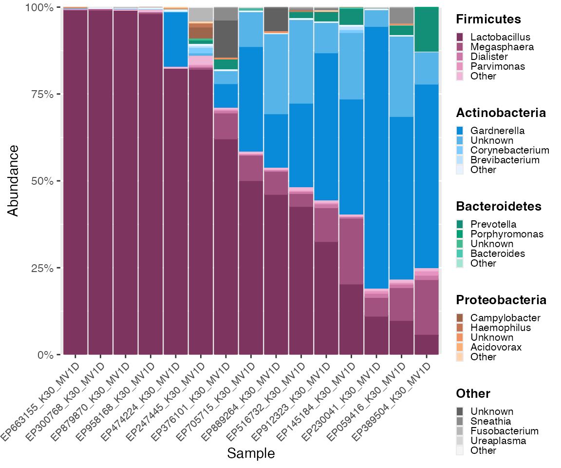

Further customization

In addition to reordering samples by abundance of a given taxon, you can supply an ordered list of samples to organize the resulting plot visually.

Apply alphabetical order

In this example, we would like to sort subject IDs alphabetically. We can achieve this by supplying a list of subject IDs in the desired order to the sample_ordering parameter.

color_objs_reorder_alpha_subject_ids <- reorder_samples_by(mdf_momspi16S,
                                                           cdf_momspi16S,
                                                           sample_variable = "short_subject_id",
                                                           sample_ordering = sort(select_ids))

mdf_reorder_alpha_ids <- color_objs_reorder_alpha_subject_ids$mdf
cdf_reorder_alpha_ids <- color_objs_reorder_alpha_subject_ids$cdf

hmp_legend_3 <- custom_legend(mdf_reorder_alpha_ids, cdf_reorder_alpha_ids)

hmp_plot_3 <- plot_microshades(mdf_reorder_alpha_ids, cdf_reorder_alpha_ids, x = "short_subject_id") +
  scale_y_continuous(labels = scales::percent, expand = expansion(0)) +
  theme(legend.position = "none") +
  theme(axis.text.x = element_text(size= 8)) +
  facet_wrap(~visit_number, scales = "free_x") +
  theme (strip.text.x = element_text(size = 8)) +
  labs(x = "Subject ID")

plot_grid(hmp_plot_3, hmp_legend_3, rel_widths = c(1, .25))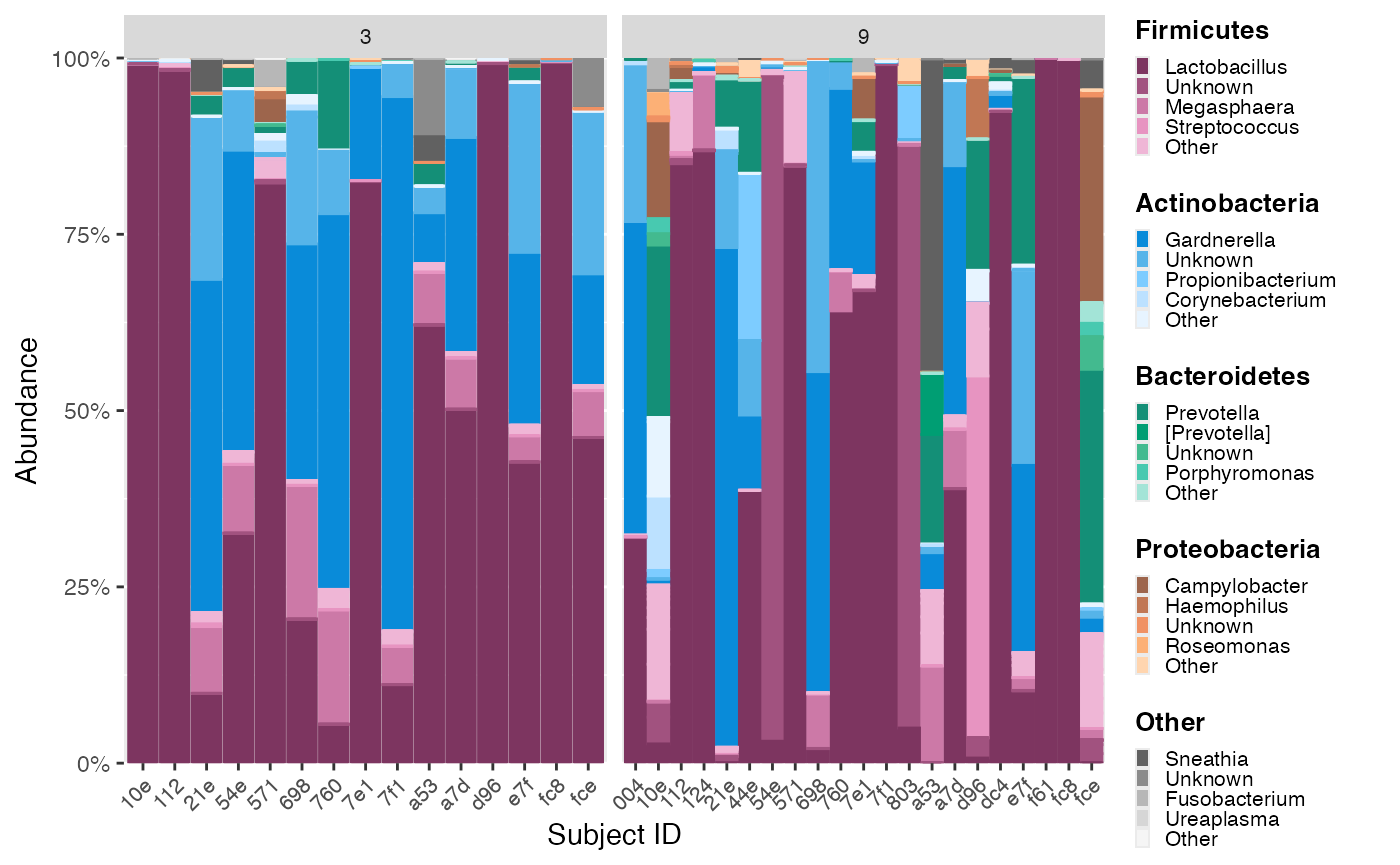

Order with narrow list

The list supplied to sample_ordering does not need to be comprised of all samples.

By default, missing samples in the list will be dropped.

If we only specify the order of samples with shortened subject IDs 004, 10e, 112, 124, and 21e, samples with other subject IDs will be dropped, and a warning will be displayed. (For using microshades in R Markdown files to generate HTMLs, warnings are able to be suppressed by setting warning=FALSE in chunk options.)

narrow_list <- c("004", "10e", "112", "124", "21e")

color_objs_reorder_narrow_subject_ids <- reorder_samples_by(mdf_momspi16S,
                                                           cdf_momspi16S,
                                                           sample_variable = "short_subject_id",
                                                           sample_ordering = narrow_list)

## Warning in reorder_samples_by(mdf_momspi16S, cdf_momspi16S, sample_variable =
## "short_subject_id", : Some samples were dropped. Check sample_ordering list.

mdf_reorder_narrow_ids <- color_objs_reorder_narrow_subject_ids$mdf
cdf_reorder_narrow_ids <- color_objs_reorder_narrow_subject_ids$cdf

hmp_legend_4 <- custom_legend(mdf_reorder_narrow_ids, cdf_reorder_narrow_ids, legend_key_size = 0.8)

hmp_plot_4 <- plot_microshades(mdf_reorder_narrow_ids, cdf_reorder_narrow_ids, x = "short_subject_id") +
  scale_y_continuous(labels = scales::percent, expand = expansion(0)) +
  theme(legend.position = "none") +
  theme(axis.text.x = element_text(size= 8)) +
  facet_grid(vars(visit_number), scales = "free_x") +
  theme (strip.text.x = element_text(size = 8), panel.spacing.y = unit(1.5, "lines")) +
  labs(x = "Subject ID")

plot_grid(hmp_plot_4, hmp_legend_4, rel_widths = c(1, .5))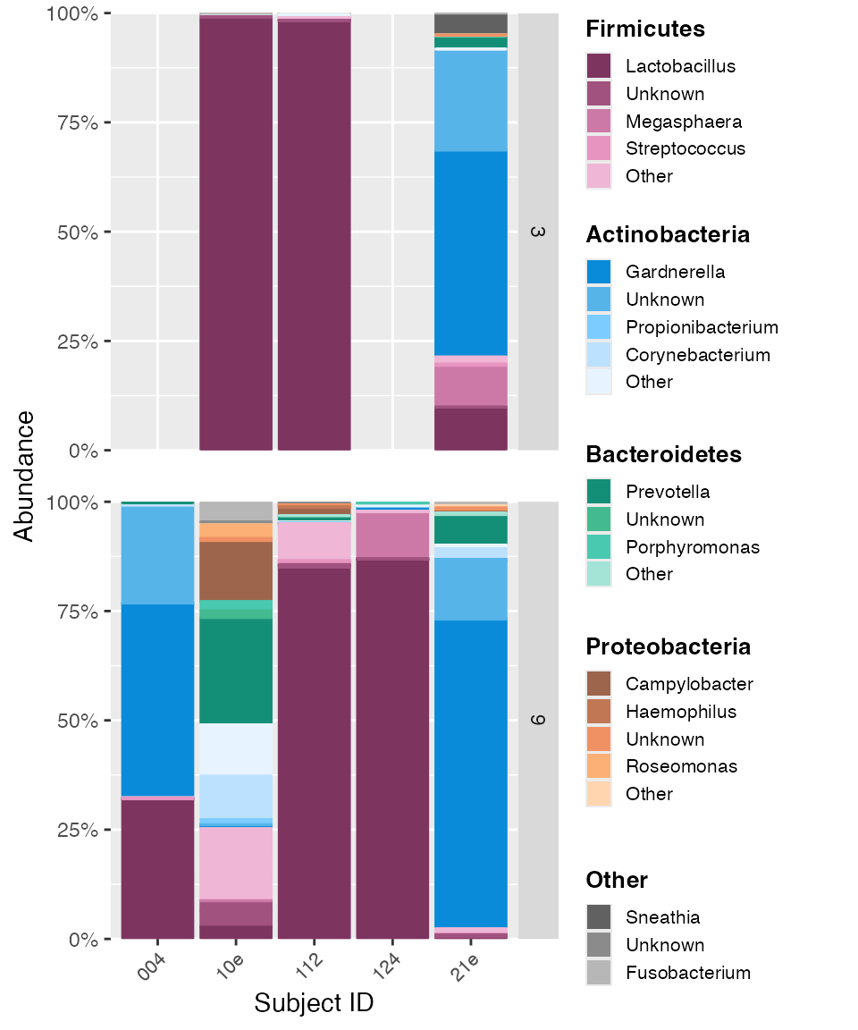

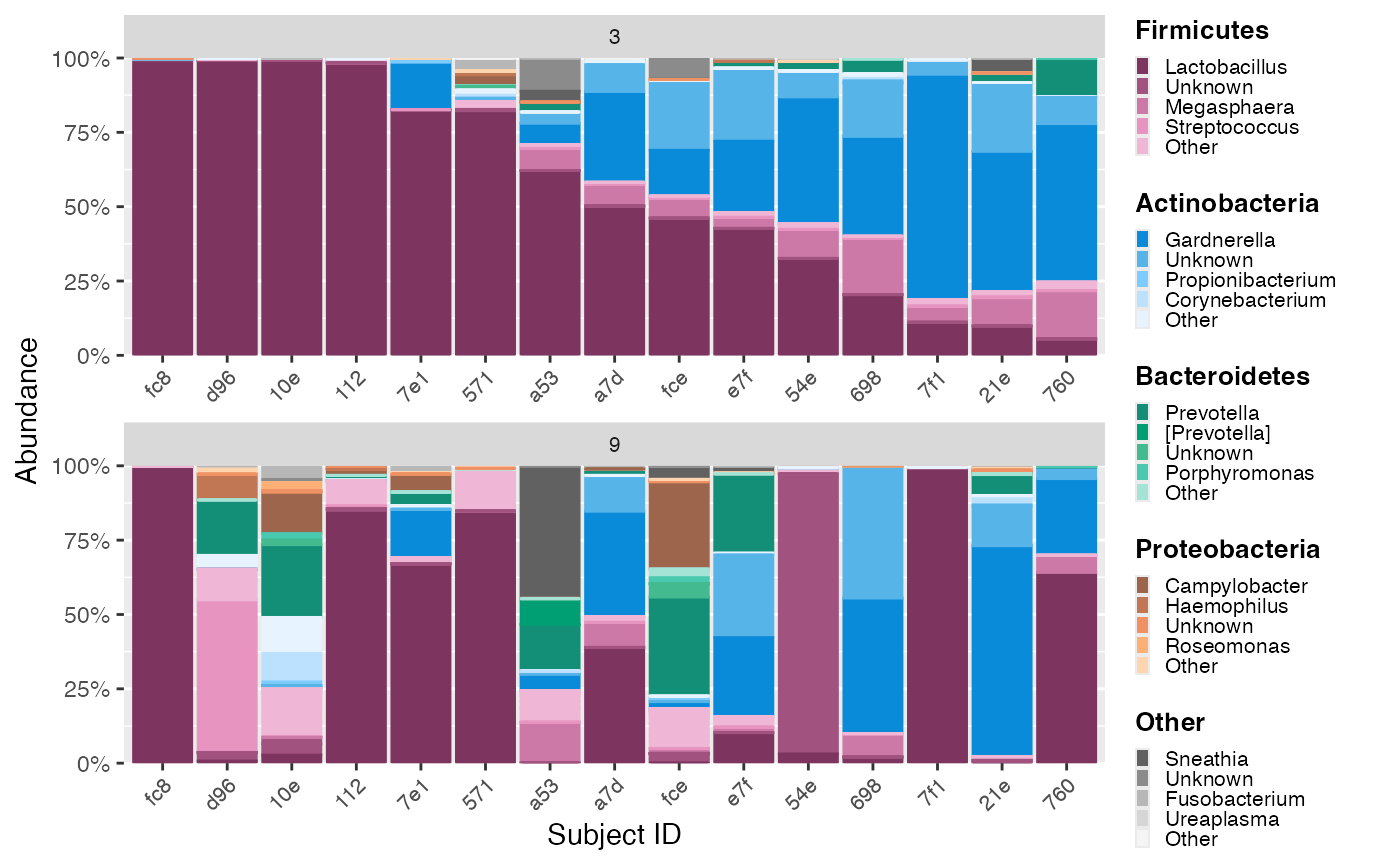
Apply abundance-based order

The reorder_samples_by function can also be used to apply existing abundance-based order to new data. Use reorder_samples_by to get the order of a sample variable, then provide this order as a list to reorder another dataset.

In this example, we would like to order by Lactobacillus abundance in Visit 3 samples, then apply this order to Visit 9 samples.

First, reorder samples from Visit 3 by Lactobacillus abundance, making sure to specify subject ID as the sample variable to sort. The resulting mdf object will be used to extract the order.

color_objs_reorder_lb_subject_ids <- reorder_samples_by(mdf_momspi16S_v3,
                                                        cdf_momspi16S_v3,
                                                        sample_variable = "short_subject_id",
                                                        order_tax = "Lactobacillus")

mdf_reorder_lb_ids <- color_objs_reorder_lb_subject_ids$mdf

Get the unique factor levels that have been set in the mdf object. Then, convert to a vector to supply to the reorder_samples_by function.

lb_desc_ids <- mdf_reorder_lb_ids %>%
                pull(short_subject_id) %>%
                fct_unique() %>%
                as.vector()

Reorder by subject ID, following the supplied order of subject IDs.

color_objs_subject_reorder_lb <- reorder_samples_by(mdf_momspi16S,
                                                    cdf_momspi16S,
                                                    sample_variable = "short_subject_id",
                                                    sample_ordering = lb_desc_ids)

## Warning in reorder_samples_by(mdf_momspi16S, cdf_momspi16S, sample_variable =
## "short_subject_id", : Some samples were dropped. Check sample_ordering list.

mdf_subject_reorder_lb <- color_objs_subject_reorder_lb$mdf
cdf_subject_reorder_lb <- color_objs_subject_reorder_lb$cdf

Compare the panels to see how the ordering of Lactobacillus abundance in Visit 3 samples has been applied to Visit 9 samples.

hmp_legend_6 <- custom_legend(mdf_subject_reorder_lb, cdf_subject_reorder_lb)

hmp_plot_6 <- plot_microshades(mdf_subject_reorder_lb, cdf_subject_reorder_lb, x = "short_subject_id") +
  scale_y_continuous(labels = scales::percent, expand = expansion(0)) +
  theme(legend.position = "none") +
  theme(axis.text.x = element_text(size= 8)) +
  facet_wrap(~visit_number, scales = "free_x", nrow=2) +
  theme (strip.text.x = element_text(size = 8)) +
  labs(x = "Subject ID")

plot_grid(hmp_plot_6, hmp_legend_6, rel_widths = c(1, .25))

Anagha Shenoy, Erin Dahl, and Lisa Karstens, PhD

June 6, 2024