Global Patterns Data
Anagha Shenoy, Erin Dahl, and Lisa Karstens, PhD
June 6, 2024
Source:vignettes/microshades-GP.Rmd
microshades-GP.RmdGlobal Patterns Data Vignette
This vignette explores the Global Patterns microbiome data available from phyloseq, which includes water samples, land samples, and human samples.
Learn more about the phyloseq package here.
Additionally, the package speedyseq is necessary to
use the function prep_mdf(). The package speedyseq provides
faster versions of phyloseq’s plotting and taxonomic merging functions.
Alternatively, the phyloseq object can be melted and transformed by
using phyloseq functions tax_glom() and/or
transform_sample_counts(), and melted by using
psmelt().
Use the microshades functions
prep_mdf
Use prep_mdf to agglomerate and normalize the phyloseq
object, and melt to a data frame. Here we specify that NA values should
be removed with the remove_na parameter, which can be
adjusted according to the needs of your visualization and analysis.
mdf_prep <- prep_mdf(GlobalPatterns, remove_na = TRUE)There is an alternative to using this function if you do not have speedyseq:
mdf_prep <- GlobalPatterns %>%
        tax_glom("Genus") %>%
        phyloseq::transform_sample_counts(function(x) { x/sum(x) }) %>%
        psmelt() %>%
        filter(Abundance > 0)
Both prep_mdf and the above option will produce the same
results.
However, prep_mdf uses the speedyseq package to increase
the speed of tax_glom and psmelt, which may be
preferable when working with large datasets.
create_color_dfs
Use create_color_dfs to generate a color object for the
specified data. Then extract the objects used to plot. mdf
represents the object to plot; cdf represents the
coloring.
color_objs_GP <- create_color_dfs(mdf_prep,
                                  selected_groups =
                                    c("Verrucomicrobia", "Proteobacteria", "Actinobacteria", "Bacteroidetes",
                                      "Firmicutes") ,
                                  cvd = TRUE)

# Extract
mdf_GP <- color_objs_GP$mdf
cdf_GP <- color_objs_GP$cdf
Plot with default parameters
Use mdf_GP as the object to plot and use
cdf_GP to assign the correct color assignments.
plot <- plot_microshades(mdf_GP, cdf_GP)

# add customizations with ggplot
plot_1 <- plot + scale_y_continuous(labels = scales::percent, expand = expansion(0)) +
  theme(legend.key.size = unit(0.2, "cm"), text=element_text(size=10)) +
  theme(axis.text.x = element_text(size= 6))

plot_1 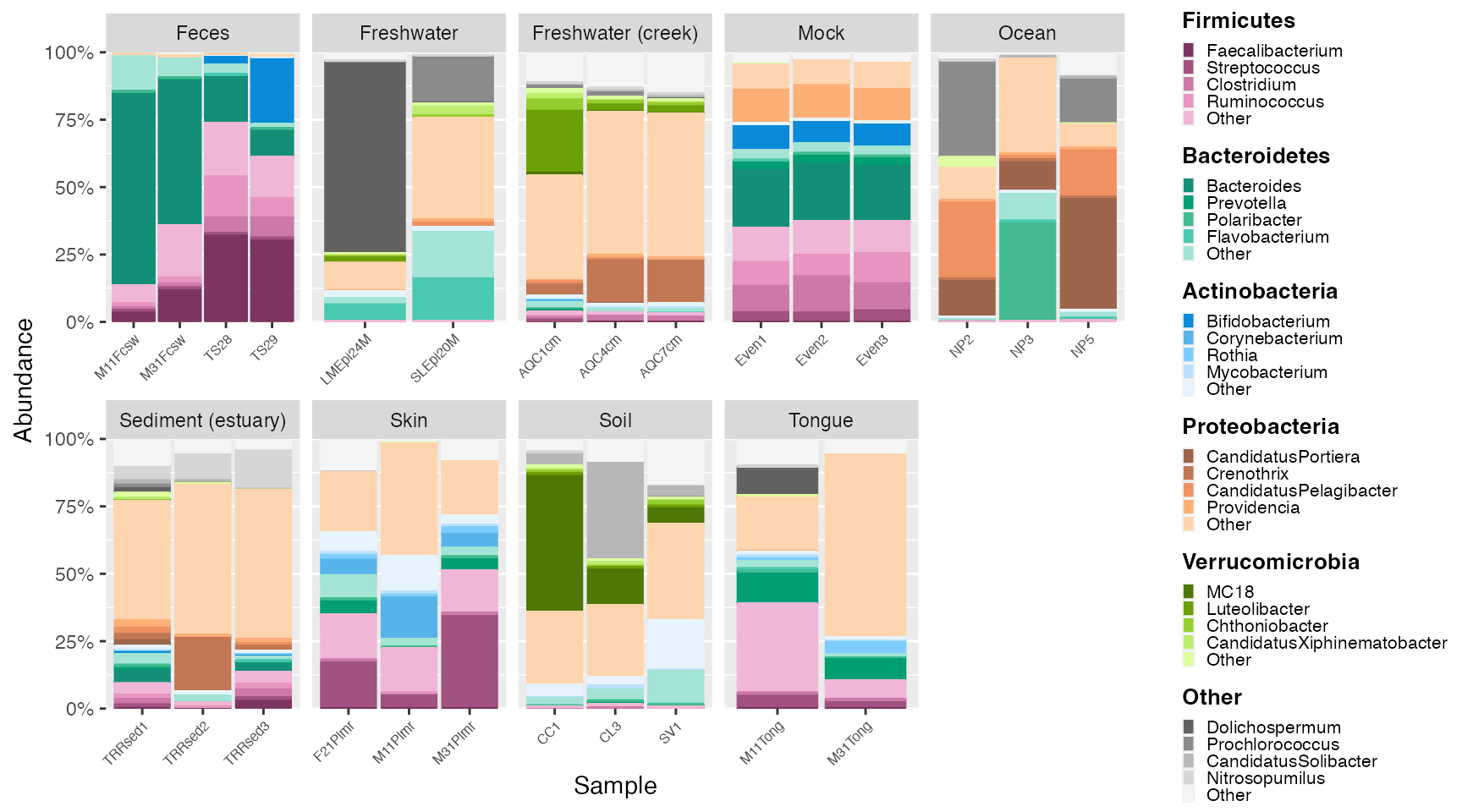
The plot_microshades returns a ggplot object, which
allows for additional specifications for the plot to be declared. For
example, this allows users to facet samples and other descriptive
elements.
plot_2 <- plot + scale_y_continuous(labels = scales::percent, expand = expansion(0)) +
  theme(legend.key.size = unit(0.2, "cm"), text=element_text(size=10)) +
  theme(axis.text.x = element_text(size= 6)) +
  facet_wrap(~SampleType, scales = "free_x", nrow = 2) +
  theme (strip.text.x = element_text(size = 6))

plot_2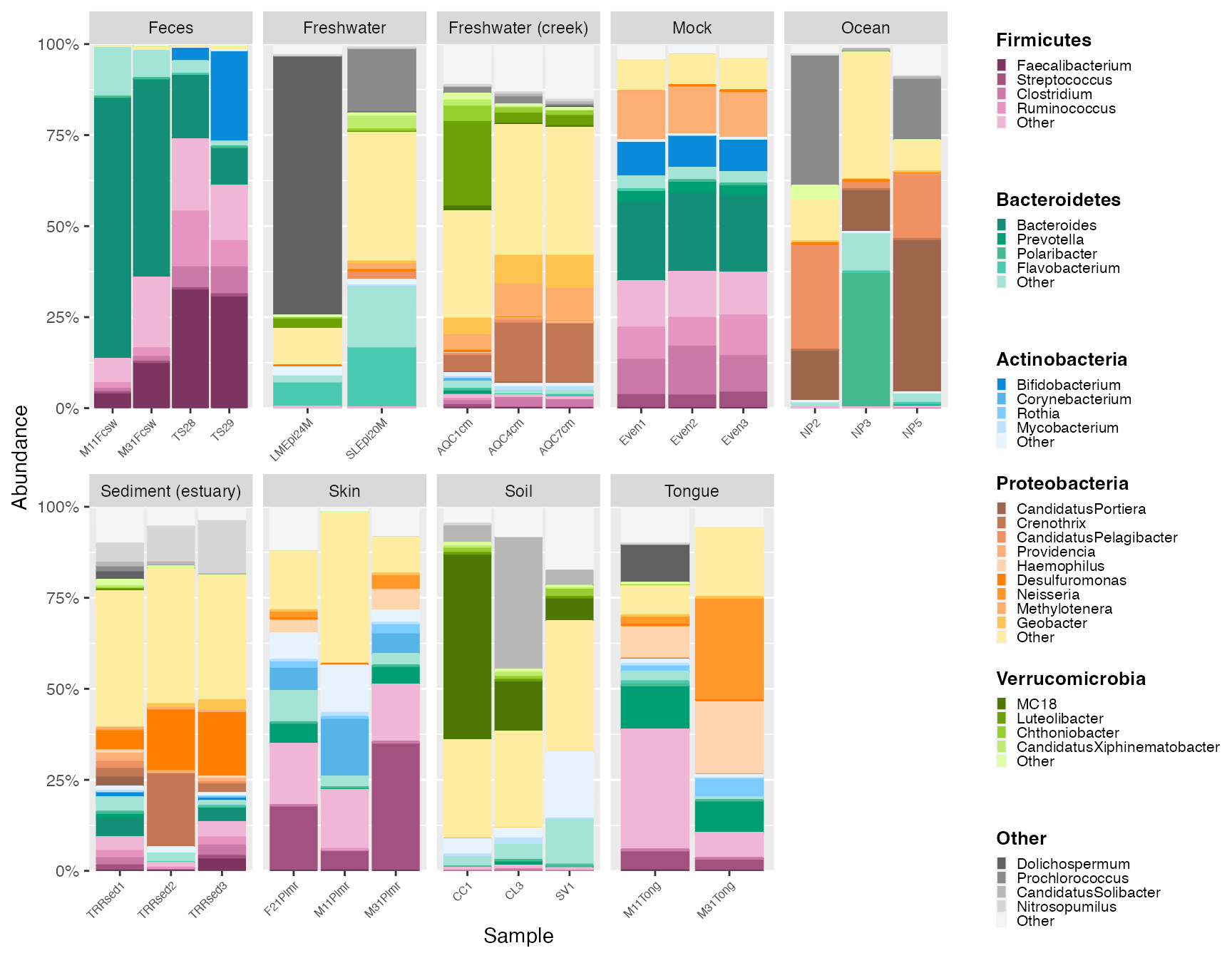
Plot with custom legend
To ensure that all elements of the custom legend are visible, adjust
legend_key_size and legend_text_size. If using
R Markdown, it may be helpful to adjust fig.height and
fig.width to receive a plot with the appropriate
dimensions.
Use plot_grid from the cowplot package to plot the
custom legend with the visualization.
To follow a detailed tutorial on how to use the
custom_legend function, see the custom
legend vignette.
GP_legend <- custom_legend(mdf_GP, cdf_GP)

plot_diff <- plot + scale_y_continuous(labels = scales::percent, expand = expansion(0)) +
  theme(legend.position = "none")  +
  theme(axis.text.x = element_text(size= 6)) +
  facet_wrap(~SampleType, scales = "free_x", nrow = 2) +
  theme(axis.text.x = element_text(size= 6)) +
  theme(plot.margin = margin(6,20,6,6))

plot_grid(plot_diff, GP_legend,  rel_widths = c(1, .25))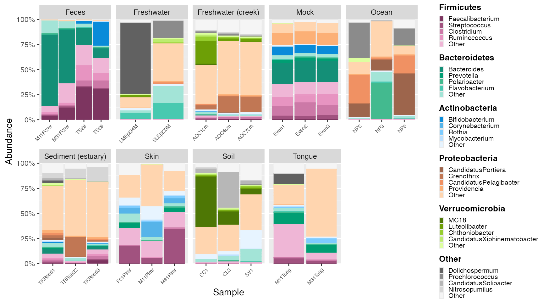
Plot with extended group colors
Here, we plot with extended Proteobacteria colors. Note the expansion of Proteobacteria groups in the legend.
new_groups <- extend_group(mdf_GP, cdf_GP, "Phylum", "Genus", "Proteobacteria", existing_palette = "micro_cvd_orange", new_palette = "micro_orange", n_add = 5)## Joining with `by = join_by(Top_Phylum, Top_Genus, group, hex)`
## Joining with `by = join_by(Top_Phylum, Top_Genus, group, hex)`
GP_legend_new <- custom_legend(new_groups$mdf, new_groups$cdf)

plot_diff <- plot_microshades(new_groups$mdf, new_groups$cdf) +
  scale_y_continuous(labels = scales::percent, expand = expansion(0)) +
  theme(legend.position = "none")  +
  theme(axis.text.x = element_text(size= 6)) +
  facet_wrap(~SampleType, scales = "free_x", nrow = 2) +
  theme(axis.text.x = element_text(size= 6)) +
  theme(plot.margin = margin(6,20,6,6))

plot_grid(plot_diff, GP_legend_new,  rel_widths = c(1, .25))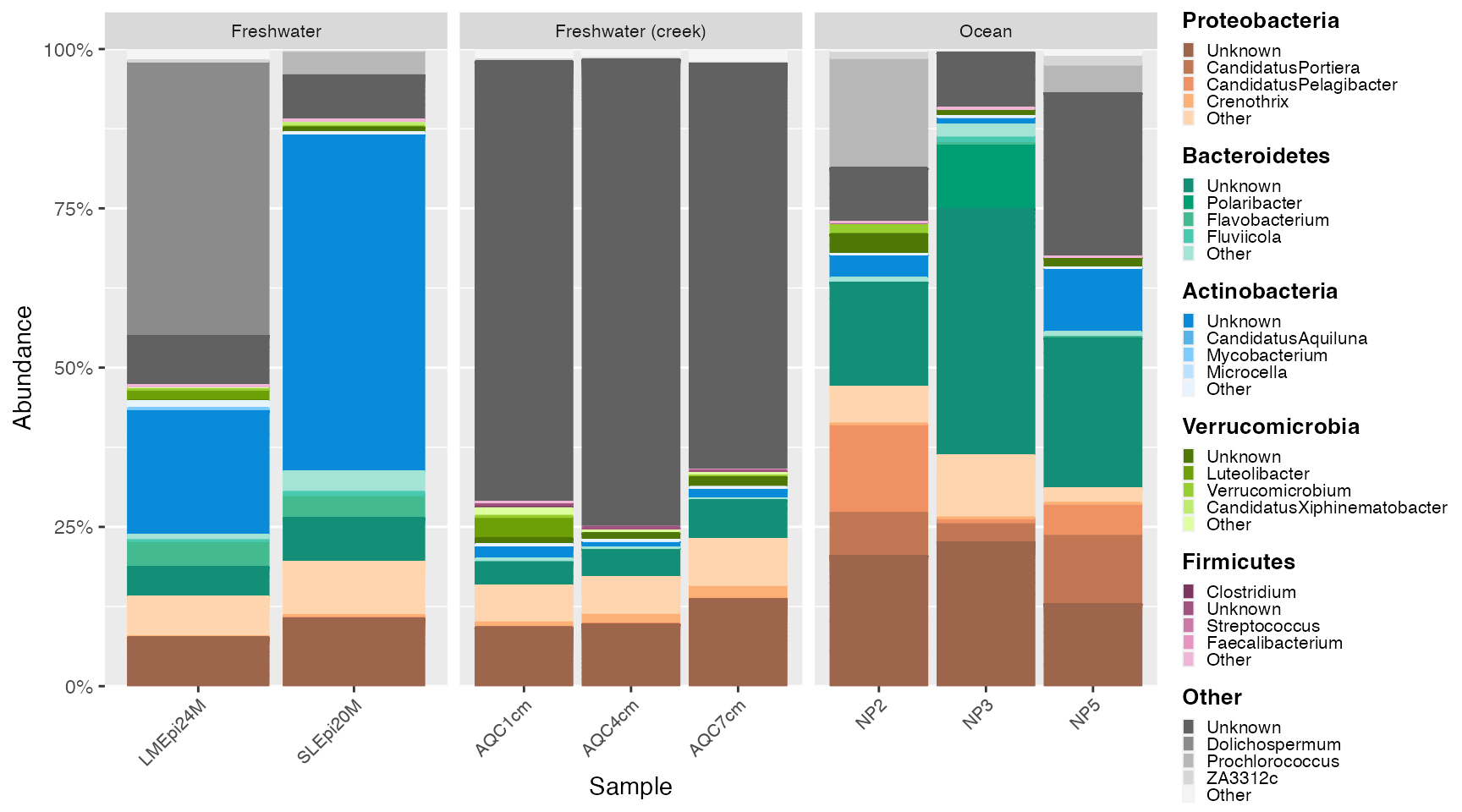
Plot subsets of data
Re-examine data with smaller groups by plotting subsets of the data. Here, we separate by sample type. Then, follow the prep → create → extract → plot sequence with each subset.
Water samples
ps_water <- subset_samples(GlobalPatterns, SampleType %in% c("Freshwater", "Freshwater (creek)", "Ocean"))

mdf_water <- prep_mdf(ps_water)

color_objs_water <- create_color_dfs(mdf_water,selected_groups = c("Verrucomicrobia", "Proteobacteria", "Actinobacteria", "Bacteroidetes",
    "Firmicutes") , cvd = TRUE)

color_objs_water <- reorder_samples_by(color_objs_water$mdf, color_objs_water$cdf)

mdf_water <- color_objs_water$mdf
cdf_water <- color_objs_water$cdf
water_legend <-custom_legend(mdf_water, cdf_water)

water_plot <- plot_microshades(mdf_water, cdf_water) +
  scale_y_continuous(labels = scales::percent, expand = expansion(0)) +
  theme(legend.position = "none") +
  theme(axis.text.x = element_text(size= 8)) +
  facet_wrap(~SampleType, scales = "free_x") +
  theme (strip.text.x = element_text(size = 8))


plot_grid(water_plot, water_legend,  rel_widths = c(1, .25))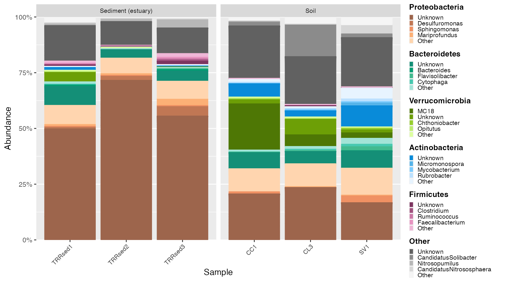
Plot contributions of water sample types
Use plot_contributions to create median and mean
abundance barplots and boxplots.
freshwater_contribution <- plot_contributions(mdf_water, cdf_water, "SampleType", "Freshwater")
creek_contribution <- plot_contributions(mdf_water, cdf_water, "SampleType", "Freshwater (creek)")
ocean_contribution <- plot_contributions(mdf_water, cdf_water, "SampleType", "Ocean")

freshwater_contribution$box +
  creek_contribution$box + theme(axis.title.y=element_blank(), axis.text.y= element_blank(), axis.ticks.y=element_blank()) +
  ocean_contribution$box + theme(axis.title.y=element_blank(), axis.text.y= element_blank(), axis.ticks.y=element_blank())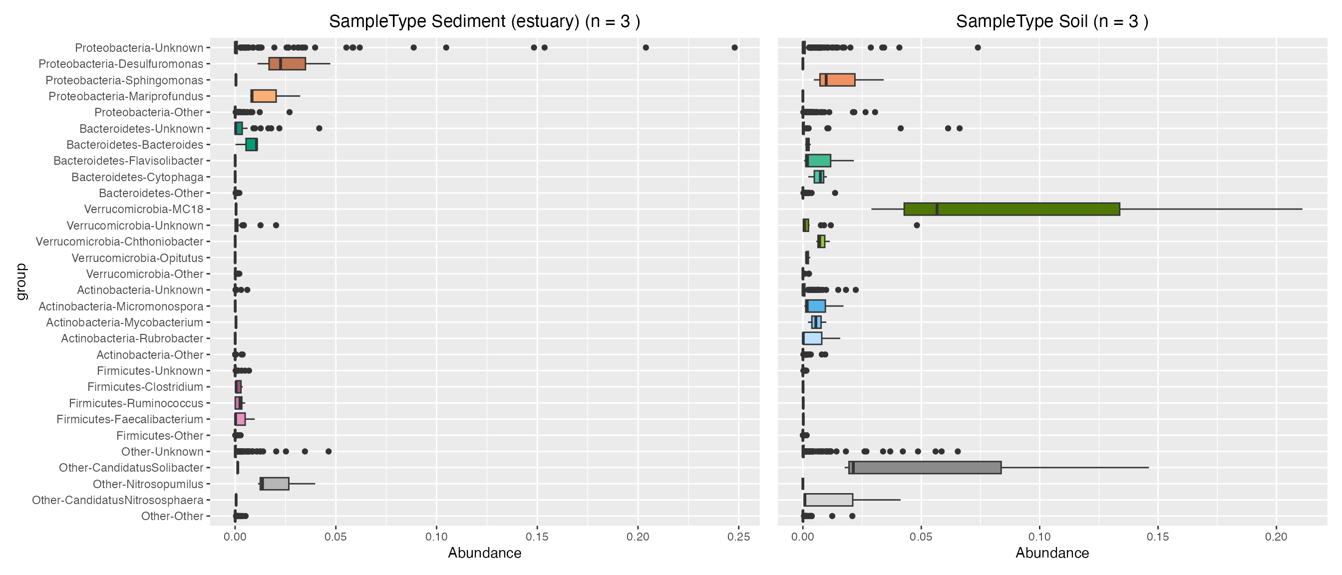
freshwater_contribution$mean +
  creek_contribution$mean + theme(axis.title.y=element_blank(), axis.text.y= element_blank(), axis.ticks.y=element_blank()) +
  ocean_contribution$mean + theme(axis.title.y=element_blank(), axis.text.y= element_blank(), axis.ticks.y=element_blank())
freshwater_contribution$median +
  creek_contribution$median + theme(axis.title.y=element_blank(), axis.text.y= element_blank(), axis.ticks.y=element_blank()) +
  ocean_contribution$median + theme(axis.title.y=element_blank(), axis.text.y= element_blank(), axis.ticks.y=element_blank())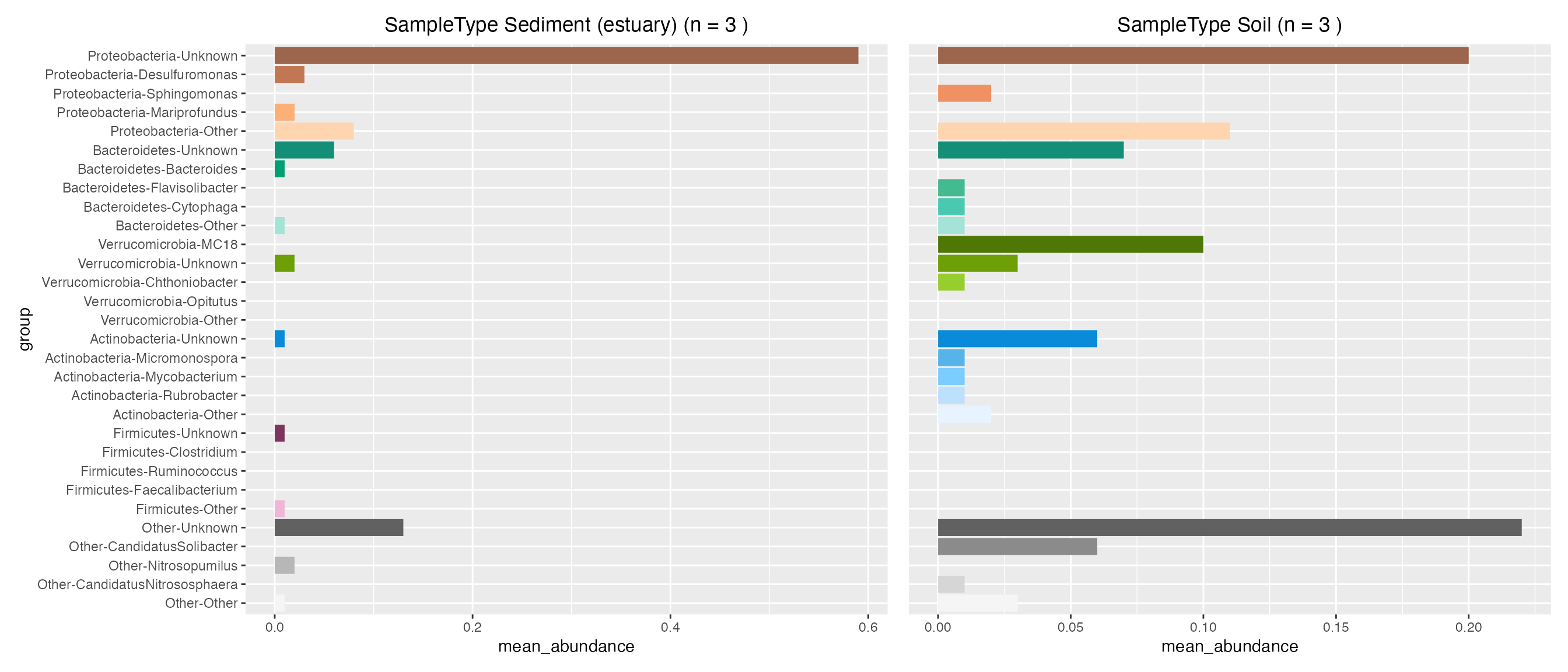
Land samples
ps_land <- subset_samples(GlobalPatterns, SampleType %in% c("Soil", "Sediment (estuary)"))

mdf_land <- prep_mdf(ps_land)
color_objs_land <- create_color_dfs(mdf_land,selected_groups = c("Verrucomicrobia", "Proteobacteria", "Actinobacteria", "Bacteroidetes",
    "Firmicutes") , cvd = TRUE)

color_objs_land <- reorder_samples_by(color_objs_land$mdf, color_objs_land$cdf)

mdf_land <- color_objs_land$mdf
cdf_land <- color_objs_land$cdf
land_legend <-custom_legend(mdf_land, cdf_land)

land_plot <- plot_microshades(mdf_land, cdf_land) +
  scale_y_continuous(labels = scales::percent, expand = expansion(0)) +
  theme(legend.position = "none") +
  theme(axis.text.x = element_text(size= 8)) +
  facet_wrap(~SampleType, scales = "free_x") +
  theme (strip.text.x = element_text(size = 8))


plot_grid(land_plot, land_legend,  rel_widths = c(1, .25))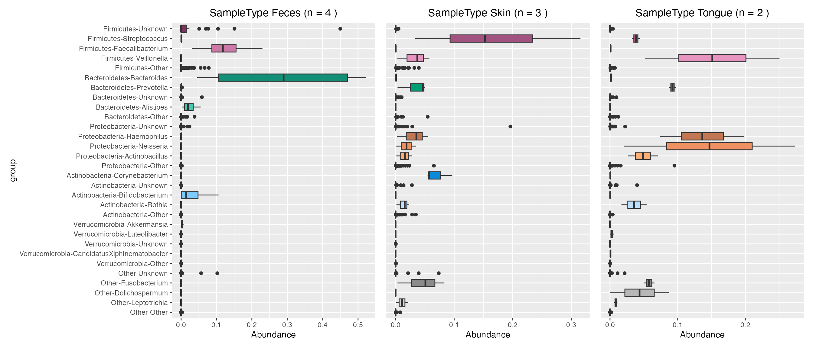
Plot contributions of land sample types
sediment_contribution <- plot_contributions(mdf_land, cdf_land, "SampleType", "Sediment (estuary)")
soil_contribution <- plot_contributions(mdf_land, cdf_land, "SampleType", "Soil")


sediment_contribution$box +
  soil_contribution$box + theme(axis.title.y=element_blank(), axis.text.y= element_blank(), axis.ticks.y=element_blank())
Human samples
ps_human <- subset_samples(GlobalPatterns, SampleType %in% c("Skin", "Feces", "Tongue"))

mdf_human <- prep_mdf(ps_human)

color_objs_human <- create_color_dfs(mdf_human,selected_groups = c("Verrucomicrobia", "Proteobacteria", "Actinobacteria", "Bacteroidetes",
    "Firmicutes") , cvd = TRUE)

color_objs_human <- reorder_samples_by(color_objs_human$mdf, color_objs_human$cdf)

mdf_human <- color_objs_human$mdf
cdf_human <- color_objs_human$cdf
human_legend <-custom_legend(mdf_human, cdf_human)

human_plot <- plot_microshades(mdf_human, cdf_human) +
  scale_y_continuous(labels = scales::percent, expand = expansion(0)) +
  theme(legend.position = "none") +
  theme(axis.text.x = element_text(size= 8)) +
  facet_wrap(~SampleType, scales = "free_x") +
  theme (strip.text.x = element_text(size = 8))


plot_grid(human_plot, human_legend,  rel_widths = c(1, .25))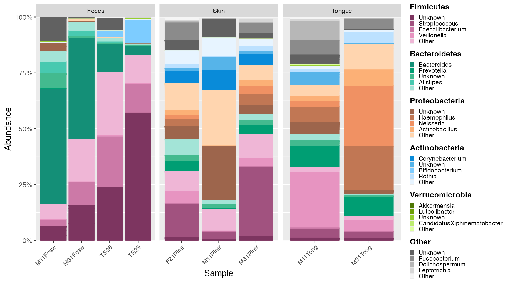
Plot contributions of human sample types
feces_contribution <- plot_contributions(mdf_human, cdf_human, "SampleType", "Feces")
skin_contribution <- plot_contributions(mdf_human, cdf_human, "SampleType", "Skin")
tongue_contribution <- plot_contributions(mdf_human, cdf_human, "SampleType", "Tongue")

feces_contribution$box +
  skin_contribution$box + theme(axis.title.y=element_blank(), axis.text.y= element_blank(), axis.ticks.y=element_blank()) +
  tongue_contribution$box + theme(axis.title.y=element_blank(), axis.text.y= element_blank(), axis.ticks.y=element_blank())