Titanic Data Example

Erin Dahl

June 6, 2024

Apply the microshades palette to Titanic data

To apply a microshades palette color to a plot, use scale_fill_manual().

The following examples use the Titanic dataset available to show how to apply the color palettes to non-microbiome data.

This first example examines the number of male and female passengers, and the class of the traveler is expressed through color shades.

library(microshades)
library(dplyr)
library(ggplot2)
 
titanic_data <- as.data.frame(Titanic)

ggplot(titanic_data, aes(x=Sex, y= Freq, fill = Class)) + 
  geom_col() +
  geom_bar(stat="identity") +
  scale_fill_manual(values = microshades_palette("micro_cvd_turquoise"))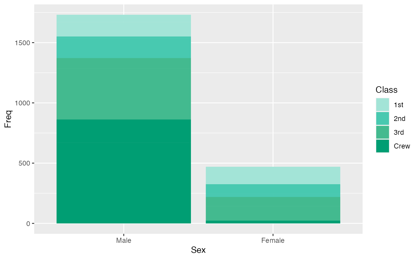

This examples compares the number of individuals who survived and how many were Adults vs. Children.

colors <- c(rev(microshades_palette("micro_blue"))[1], rev(microshades_palette("micro_purple"))[1])

ggplot(titanic_data, aes(x=Survived, y= Freq, fill = Age)) + 
  geom_bar(position=position_dodge(), stat="identity") +
  scale_fill_manual(values = colors )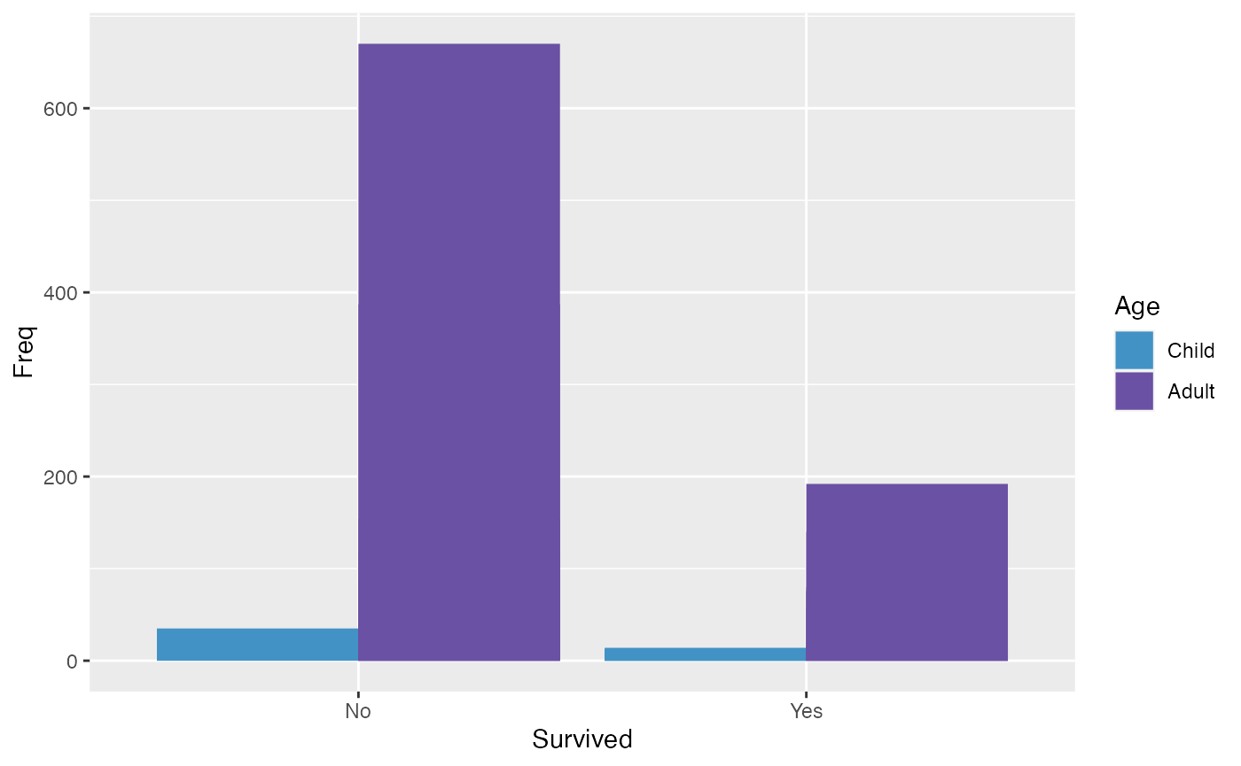

This plot shows the number of Child vs. Adult passengers, and their respective classes.

ggplot(titanic_data, aes(x=Age, y= Freq, fill = Class)) + 
  geom_bar(position=position_dodge(), stat="identity") +
  scale_fill_manual(values = microshades_palette("micro_cvd_purple"))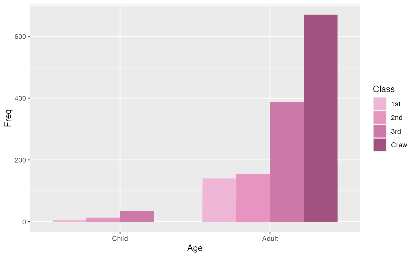

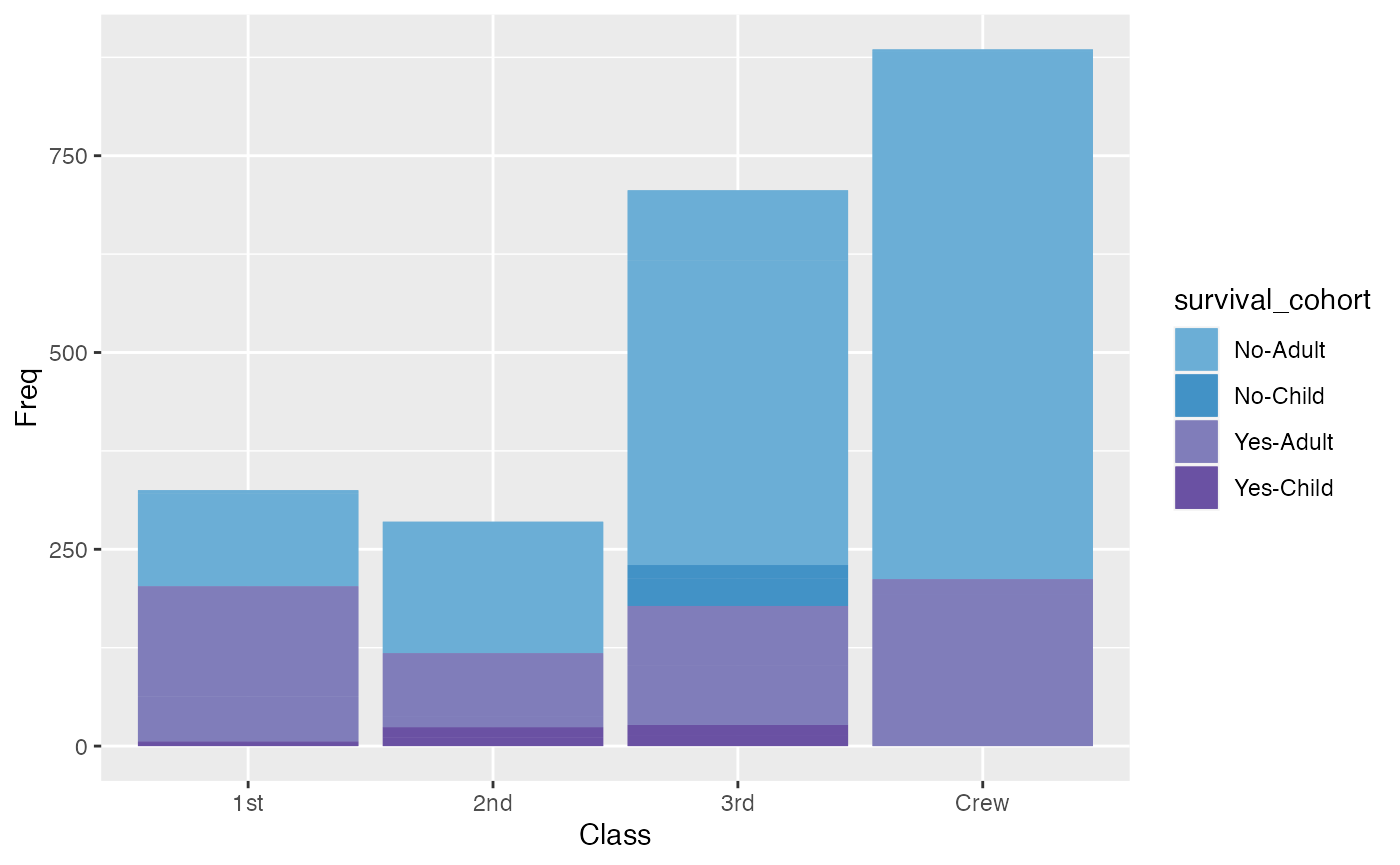
For the plot below, a combination variable that combines Survival and Age categories is created and called the survival cohort. This variable allows for a more detailed coloring of the plot.

titanic_mod <- titanic_data %>% mutate(survival_cohort = paste(Survived, Age, sep = "-"))
colors <-c(microshades_palette("micro_blue", 2, lightest = FALSE), 
           microshades_palette("micro_purple", 2, lightest = FALSE))


ggplot(titanic_mod, aes(x=Class, y= Freq, fill = survival_cohort)) + 
  geom_col() +
  geom_bar(stat="identity") +
  scale_fill_manual(values = colors)