Remove NA Option

The microshades package allows for color organization in data visualizations, particularly visualizations of microbiome data. Relative abundance plots are common to microbiome investigations as they present an informative overview of the bacterial composition of samples.

Previously, the default microshades behavior in versions 1.1 and earlier was such that NA values in the input data (a phyloseq object) were ignored. That is, relative abundances were calculated as though bacteria that are not identified taxonomically are not present in the sample. For more details on the issue and origin of the behavior, see issue 18.

The default behavior of microshades in versions 1.11 and later is NOT to remove NA values. If users wish to remove NAs , the prep_mdf function has a remove_na parameter to allow users to specify whether or not NA values should be removed from the data during the taxa agglomeration step.

Removal of NA values can affect interpretation of data depending on what dataset is examined. The following example demonstrates this in addition to demonstrating how to remove NAs when using microshades.

Load packages & data

library(microshades)
library(phyloseq)
library(ggplot2)
library(dplyr)
library(cowplot)
library(patchwork)
library(forcats)

# The dataset Global Patterns is a phyloseq object available from the Phyloseq package
data(GlobalPatterns)

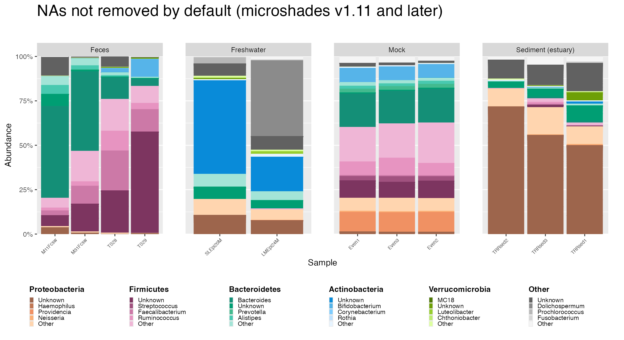
Code to generate default plot with NAs

mdf_GP_updated is the object to be plotted. It contains the abundance information organized by taxa (phylum and genus in this example), with NA values not removed. cdf_GP_updated will be used for coloring the plot.

mdf_updated <- prep_mdf(GlobalPatterns) # prep_mdf function to agglomerate, normalize, melt

# Create abundance dataframe & color mapping dataframe
color_objs_GP_updated <- create_color_dfs(mdf_updated, 
                                  selected_groups = 
                                    c("Verrucomicrobia", "Proteobacteria", "Actinobacteria", "Bacteroidetes",
                                    "Firmicutes"),
                                  cvd = TRUE)

mdf_GP_updated <- color_objs_GP_updated$mdf
cdf_GP_updated <- color_objs_GP_updated$cdf

# Order the samples by Proteobacteria abundance for visual organization
reordered_GP_update <- reorder_samples_by(mdf_GP_updated, 
                                          cdf_GP_updated, 
                                          order = "Proteobacteria", 
                                          group_level = "Phylum", 
                                          subgroup_level = "Genus", 
                                          sink_abundant_groups = TRUE)

# Extract dataframes
mdf_up_GP <- reordered_GP_update$mdf
cdf_up_GP <- reordered_GP_update$cdf

mdf_up_GP <- mdf_up_GP %>% subset(SampleType %in% c("Feces", "Freshwater", "Mock", "Sediment (estuary)"))

legend <- custom_legend(mdf_up_GP, cdf_up_GP, legend_orientation = "horizontal")
center_legend <- plot_grid(NULL, legend, nrow=1, rel_widths=c(0.04, 0.96))

plot_updated <- plot_microshades(mdf_up_GP, cdf_up_GP)

faceted_plot_updated <- plot_updated + 
  scale_y_continuous(labels = scales::percent, expand = expansion(0)) +
  theme(legend.position="none") +
  facet_wrap(~SampleType, scales = "free_x", ncol=4) +
  theme(axis.text.x = element_text(size = 6)) +
  theme(plot.margin = margin(6,20,6,6)) +
  theme(plot.title = element_text(size = 20, margin=margin(0,0,30,0))) +
  theme(panel.spacing = unit(2, "lines")) +
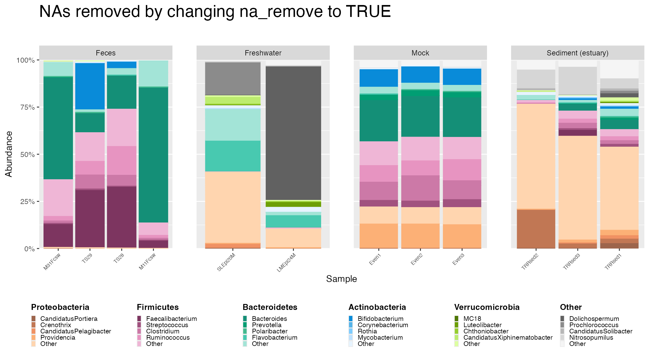
  ggtitle("NAs not removed by default (microshades v1.11 and later)")

Code to generate plot with NAs removed

To remove NAs, the remove_NA parameter is set to TRUE when calling the prep_mdf function.

mdf_prep <- prep_mdf(GlobalPatterns, remove_na = TRUE) # NAs to be removed

# Create abundance dataframe & color mapping dataframe
color_objs_GP <- create_color_dfs(mdf_prep, 
                                  selected_groups = 
                                    c("Verrucomicrobia", "Proteobacteria", "Actinobacteria", "Bacteroidetes",
                                    "Firmicutes"),
                                  cvd = TRUE)

# Extract dataframes
mdf_GP <- color_objs_GP$mdf
cdf_GP <- color_objs_GP$cdf

# Order the samples by Proteobacteria abundance for visual organization
reordered_GP <- reorder_samples_by(mdf_GP, 
                                   cdf_GP, 
                                   order = "Proteobacteria", 
                                   group_level = "Phylum", 
                                   subgroup_level = "Genus", 
                                   sink_abundant_groups = TRUE)

# Extract dataframes
mdf_re_GP <- reordered_GP$mdf
cdf_re_GP <- reordered_GP$cdf

mdf_re_GP <- mdf_re_GP %>% subset(SampleType %in% c("Feces", "Freshwater", "Mock", "Sediment (estuary)"))

facet_legend <- custom_legend(mdf_re_GP, cdf_re_GP, legend_orientation = "horizontal")
center_facet_legend <- plot_grid(NULL, facet_legend, nrow=1, rel_widths=c(0.04, 0.96))

plot <- plot_microshades(mdf_re_GP, cdf_re_GP)

faceted_plot <- plot + 
  scale_y_continuous(labels = scales::percent, expand = expansion(0)) +
  theme(legend.position="none") +
  facet_wrap(~SampleType, scales = "free_x", ncol = 4) +
  theme(axis.text.x = element_text(size = 6)) +
  theme(plot.margin = margin(6,20,6,6)) +
  theme(plot.title = element_text(size = 20, margin=margin(0,0,30,0))) +
  theme(panel.spacing = unit(2, "lines")) +
  ggtitle("NAs removed by changing na_remove to TRUE")

Visual comparison of NA removal

Note that the relative abundances present differently when the NA values are removed.

plot_grid(faceted_plot_updated, center_legend, rel_heights = c(1, .25), nrow=2)

plot_grid(faceted_plot, center_facet_legend, rel_heights = c(1, .25), nrow=2)

Anagha Shenoy, Lisa Karstens

August 25, 2023

Load packages & data

Code to generate default plot with NAs

Code to generate plot with NAs removed

Visual comparison of NA removal